Perspectives


Sustainable Design: Our commitment and plan to design responsibly for the future
At LEO A DALY, we hold the long view on sustainable design as responsible design, and that’s why we are signatories of all industry commitments on sustainability. The responsible use of resources translates to long term returns for our clients and communities through high performance buildings, improved open space, and healthy interior environments. Sustainability is a core value of LEO A DALY, and the firm has championed sustainable practices and materials across the markets it operates in.
In climate disasters, resilient design serves the entire community
By efficiently storing, managing, and distributing food resources, these centers help stabilize food availability after extreme weather events. In times of crisis, the importance of these centers cannot be overstated, as they are key to not only feeding populations but also supporting community recovery and fostering long-term environmental stewardship.
Decarbonization: Challenges and Opportunities in Reducing Embodied Carbon
As climate change urgency grows, reducing embodied carbon in buildings becomes crucial for creating a sustainable built environment, achieved by using materials with lower carbon footprints throughout their lifecycle.
Future-Proofing the Past through Adaptive Reuse
Uncover the technologies and skills needed to enable adaptive reuse that transforms old buildings into sustainable spaces.
Lighting and Sustainability Facilitate ‘Doing Good’ at Thurgood Marshall Hall
Thurgood Marshall Hall, home to the School of Public Policy at the University of Maryland, stands at the heart of a new entrance to campus as a highly visible symbol of the university’s dedication to serving the public good. Our design team incorporated a wide variety of sustainability features into this LEED® Gold building, and wellness was a special focus.
Materials Matter: Evaluating the Impact of Building Materials
Understanding the full impact of building materials is complex and requires strategies to identify products and material selections that consider all living systems.
Four Technologies Airports Can Implement Now to Become More Sustainable
As customers increasingly expect sustainability features from their airports, here are four infrastructure upgrades that are feasible, budget-friendly and offer a positive impact on carbon emissions.
Inspired by Opportunity: First-year Experiences at LEO A DALY
Young design professionals across the firm share their first-year experience at LEO A DALY.
Creating access to critical care through hospital expansion
LEO A DALY Healthcare designers discuss the complex process of hospital expansion in a 28-phase Cardiovascular Suite Relocation for M Health Fairview to bring tertiary cardiac care to more patients in the Minneapolis metro.
Resiliency Roadmap: Design Strategies for Resilient Buildings
What is resilience? It's the ability to adapt to changing conditions and maintain or regain functionality and vitality in the face of stress or disturbance. Stress or disturbance could be a hurricane, earthquake or some other natural phenomenon.
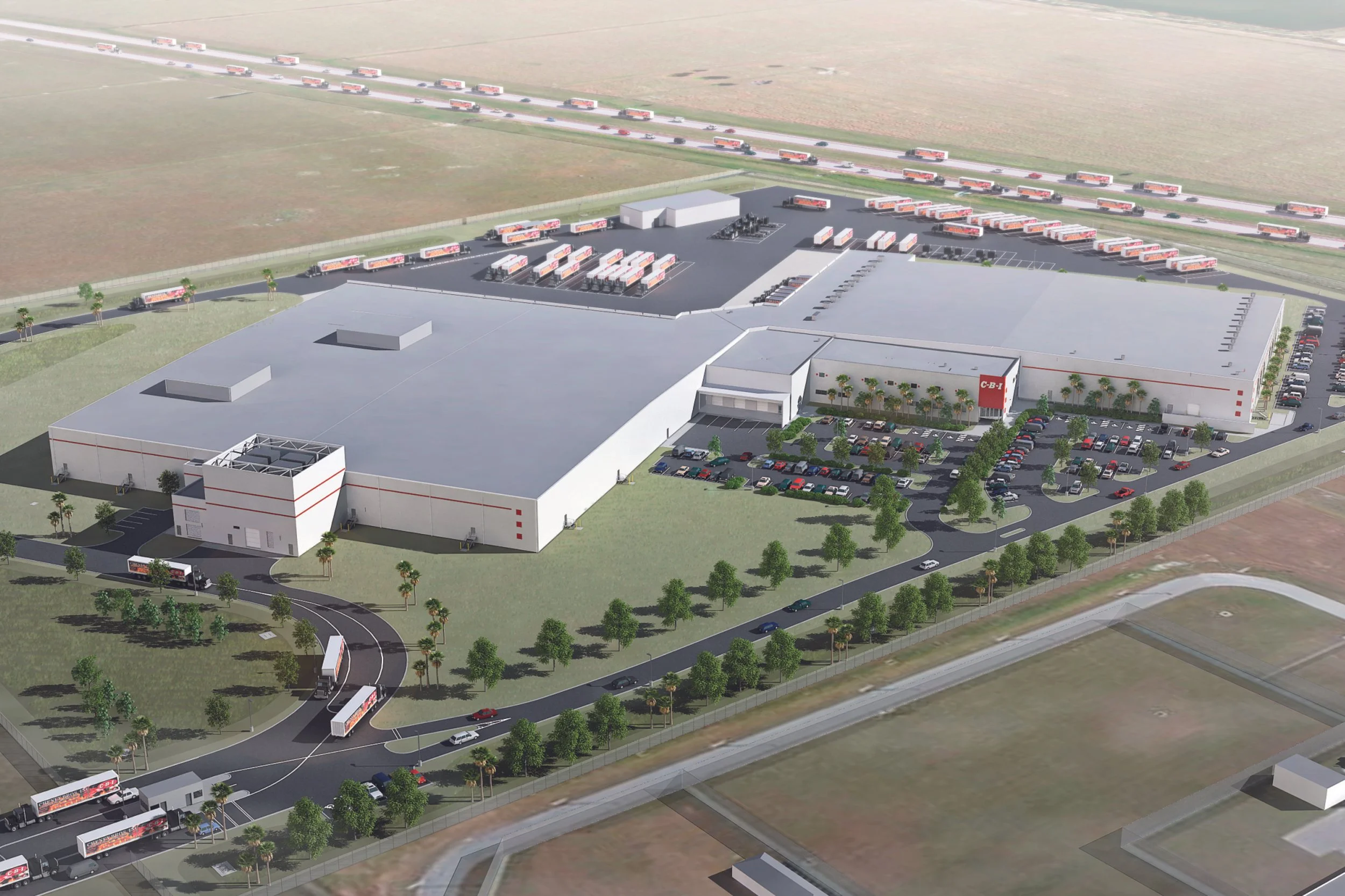
Resilient design proved critical to Hurricane Ian relief efforts
Designed for resilience, the Cheney Bros food-distribution warehouse in Punta Gorda, Florida, more than weathered the storm. It provided safe harbor.
Designing for dignity in senior living
Senior Living Practice Leader Mike Rodebaugh, AIA, explores the complex and meaningful craft of dignity-driven design.
Resort Style Senior Living in Boca Raton
Sinai Residences in Boca Raton sets the standard for continuing care communities in South Florida via Dignity Driven Design.
Bringing pro sports to Las Vegas
The rebirth of Las Vegas as a sports destination shows how designers, city planners and visionary clients can unite to transform a city.
Climate justice is the design challenge of our lives
Climate change and toxic emissions disproportionately affect poor and minority communities. Here's how designers can help.

"Illuminating" South Sioux City Marriott Riverfront
An integrated approach to lighting design helps LEO A DALY and Reveal Design Group create unforgettable hospitality experiences